Welcome to LLSpy’s documentation!

LLSpy: Lattice light-sheet post-processing utility

Copyright © 2017 Talley Lambert, Harvard Medical School.

LLSpy is a python library to facilitate lattice light sheet data processing. It extends the cudaDeconv binary created in the Betzig lab at Janelia Research Campus, adding features that auto-detect experimental parameters from the data folder structure and metadata (minimizing user input), auto-choose OTFs, perform image corrections and manipulations, and facilitate file handling.

Introduction

Overview

LLSpy is a python library to facilitate lattice light sheet data processing. It extends the cudaDeconv binary created in the Betzig lab at Janelia Research Campus, adding features that auto-detect experimental parameters from the data folder structure and metadata (minimizing user input), auto-choose OTFs, perform image corrections and manipulations, and facilitate file handling. Full(er) documentation available at http://llspy.readthedocs.io/

There are three ways to use LLSpy:

1. Graphical User Interface

The GUI provides access to the majority of functionality in LLSpy. It includes a drag-and drop queue, visual progress indicator, and the ability to preview data processed with the current settings using the (awesome) 4D-viewer, Spimagine developed by Martin Weigert in the Myers lab at MPI-CBG. Support for online-processing with a “monitored folder” or real-time visualization with Spimagine is in development.

GUI documentation here.

2. Command Line Interface

The command line interface can be used to process LLS data in a server environment (linux compatible).

$ lls --help

Usage: lls [OPTIONS] COMMAND [ARGS]...

  LLSpy

  This is the command line interface for the LLSpy library, to facilitate
  processing of lattice light sheet data using cudaDeconv and other tools.

Options:
  --version          Show the version and exit.
  -c, --config PATH  Config file to use instead of the system config.
  --debug
  -h, --help         Show this message and exit.

Commands:
  camera    Camera correction calibration
  clean     Delete LLSpy logs and preferences
  compress  Compression & decompression of LLSdir
  config    Manipulate the system configuration for LLSpy
  decon     Deskew and deconvolve data in LLSDIR.
  deskew    Deskewing only (no decon) of LLS data
  gui       Launch LLSpy Graphical User Interface
  info      Get info on an LLSDIR.
  install   Install cudaDeconv libraries and binaries
  reg       Channel registration

# process a dataset
$ lls decon --iters 8 --correctFlash /path/to/dataset

# change system or user-specific configuration
$ lls config --set otfDir path/to/PSF_and_OTFs

# or launch the gui
$ lls gui

Command line documentation here.

3. Interactive data processing in a python console

 >>> import llspy

 # the LLSdir object contains most of the useful attributes and
 # methods for interacting with a data folder containing LLS tiffs
 >>> E = llspy.LLSdir('path/to/experiment_directory')
 # it parses the settings file into a dict:
 >>> E.settings
 {'acq_mode': 'Z stack',
  'basename': 'cell1_Settings.txt',
  'camera': {'cam2name': '"Disabled"',
             'cycle': '0.01130',
             'cycleHz': '88.47 Hz',
             'exp': '0.01002',
     ...
 }

 # many important attributes are in the parameters dict
 >>> E.parameters
 {'angle': 31.5,
  'dx': 0.1019,
  'dz': 0.5,
  'nc': 2,
  'nt': 10,
  'nz': 65,
  'samplescan': True,
   ...
 }

 # and provides methods for processing the data
 >>> E.autoprocess()

 # the autoprocess method accepts many options as keyword aruguments
 # a full list with descriptions can be seen here:
 >>> llspy.printOptions()

               Name  Default                    Description
               ----  -------                    -----------
       correctFlash  False                      do Flash residual correction
 flashCorrectTarget  cpu                        {"cpu", "cuda", "parallel"} for FlashCor
             nIters  10                         deconvolution iters
          mergeMIPs  True                       do MIP merge into single file (decon)
             otfDir  None                       directory to look in for PSFs/OTFs
             tRange  None                       time range to process (None means all)
             cRange  None                       channel range to process (None means all)
                ...  ...                        ...

# as well as file handling routines
>>> E.compress(compression='lbzip2')  # compress the raw data into .tar.(bz2|gz)
>>> E.decompress()  # decompress files for re-processing
>>> E.freeze()  # delete all processed data and compress raw data for long-term storage.

API documentation here.

Features of LLSpy

• graphical user interface with persistent/saveable processing settings
• command line interface for remote/server usage (coming)
• preview processed image to verify settings prior to processing full experiment
• Pre-processing corrections:
  • correct “residual electron” issue on Flash4.0 when using overlap synchronous mode. Includes CUDA and parallel CPU processing as well as GUI for generation of calibration file.
  • apply selective median filter to particularly noisy pixels
  • trim image edges prior to deskewing (helps with CMOS edge row artifacts)
  • auto-detect background
• Processing:
  • select subset of acquired images (C or T) for processing
  • automatic parameter detection based on auto-parsing of Settings.txt
  • automatic OTF generation/selection from folder of raw PSF files, based on date of acquisition, mask used (if entered into SPIMProject.ini), and wavelength.
  • graphical progress bar and time estimation
• Post-processing:
  • proper voxel-size metadata embedding (newer version of Cimg)
  • join MIP files into single hyperstack viewable in ImageJ/Fiji
  • automatic width/shift selection based on image content (“auto crop to features”)
  • automatic fiducial-based image registration (provided tetraspeck bead stack)
  • compress raw data after processing
• Watched-folder autoprocessing (experimental):
  • Server mode: designate a folder to watch for incoming finished LLS folders (with Settings.txt file). When new folders are detected, they are added to the processing queue and the queue is started if not already in progress.
  • Aquisition mode: designed to be used on the aquisition computer. Designate folder to watch for new LLS folders, and process new files as they arrive. Similar to built in GPU processing tab in Lattice Scope software, but with the addition of all the corrections and parameter selection in the GUI.
• easily return LLS folder to original (pre-processed) state
• compress and decompress folders and subfolders with lbzip2 (not working on windows)
• concatenate two experiments - renaming files with updated relative timestamps and stack numbers
• rename files acquired in script-editor mode with Iter_ in the name to match standard naming with positions (work in progress)
• cross-platform: includes precompiled binaries and shared libraries that should work on all systems.

Requirements

• Compatible with Windows (tested on 7/10), Mac or Linux (tested on Ubuntu 16.04)
• Python 3.6 (recommended), 3.5, or 2.7
• Most functionality assumes a data folder structure as generated by the Lattice Scope LabeView acquisition software written by Dan Milkie in the Betzig lab. If you are using different acquisition software, it is likely that you will need to change the data structure and metadata parsing routines.
• Currently, the core deskew/deconvolution processing is based on cudaDeconv, written by Lin Shao and maintained by Dan Milkie. cudaDeconv is licensed and distributed by HHMI. It is not included in this repository and must be acquired seperately in the dropbox share accessible after signing the RLA with HHMI. Contact innovation@janlia.hhmi.org.
• CudaDeconv requires a CUDA-capable GPU
• The Spimagine viewer requires a working OpenCL environment

Installation

Note: As of version 0.4.2 cudaDecon is now included in the LLSpy conda package and requires no additional steps for installation. Horray for open source!

1. Install Anaconda or Miniconda

2. Launch a terminal window (OS X, Linux), or Anaconda Prompt (Windows)

3. Add the “conda-forge” and “talley” channels to your conda config

   $ conda config --add channels conda-forge
   $ conda config --add channels talley
   

4. Install LLSpy into a new conda environment

   $ conda create -n llsenv python=3.6 llspy
   $ conda activate llsenv
   

   The create -n llsenv line creates a virtual environment. This is optional, but recommended as it easier to uninstall cleanly and prevents conflicts with any other python environments. If installing into a virtual environment, you must source the environment before proceeding, and each time before using llspy.

Each time you use the program, you will need to activate the virtual environment. The main command line interface is lls, and the gui can be launched with lls gui. You can create a bash script or batch file to autoload the environment and launch the program if desired.

# Launch Anaconda Prompt and type...
$ conda activate llsenv

# show the command line interface help menu
$ lls -h
# process a dataset
$ lls decon /path/to/dataset
# or launch the gui
$ lls gui

Setup

There are a few things that must be configured properly in order for LLSpy to work.

OTF Directory

Important

LLSpy is currently limited to PSF/OTF files that were acquired in galvo/objective scanning mode, using a 0.1µm Z step size. This assumption is made both during generation of OTFs from PSF files in the OTF directory, and during deconvolution made with pre-generated OTF files. So even if you have made OTF files manually (using, for example, radialft), the voxel size must still be 0.1µm. This is a limitation that will eventually be fixed, but feel free to raise a github issue if you require this flexibility.

LLSpy assumes that you have a directory somewhere with all of your PSF and OTF files. You must enter this directory on the config tab of the LLSpy gui or by using lls config --set otfDir PATH in the command line interface.

The simplest setup is to create a directory and include an OTF for each wavelength you wish to process, for instance:

/home/myOTFs/
├── 405_otf.tif
├── 488_otf.tif
├── 560_otf.tif
├── 642_otf.tif

The number in the filenames comes from the wavelength of the laser used for that channel. This is parsed directly from the filenames, which in turn are generated based on the name of the laser lines specified in the SPIMProject AOTF.mcf file in the SPIM Support Files directory of the Lattice Scope software. For instance, if an AOTF channel is named “488nm-SB”, then an example file generated with that wavelength might be called:

cell5_ch0_stack0000_488nm-SB_0000000msec_0020931273msecAbs.tif

The parsed wavelength will be the digits only from the segment between the stack number and the relative timestamp. In this case: “488nm-SB” –> “488”. For more detail on filename parsing see filename parsing below.

As a convenience, you can also place raw PSF files in this directory with the following naming convention:

[date]_[wave]_[slm_pattern]_[outerNA]-[innerNA].tif

… where outerNA and innerNA use ‘p’ instead of decimal points, for instance:

20160825_488_square_0p5-0p42.tif

the actual regex that parses the OTF is as follows

psffile_pattern = re.compile(
    r"""
    ^(?P<date>\d{6}|\d{8})      # 6 or 8 digit date
    _(?P<wave>\d+)              # wavelength ... only digits following _ are used
    _(?P<slmpattern>[a-zA-Z_]+)  # slm pattern
    _(?P<outerNA>[0-9p.]+)      # outer NA, digits with . or p for decimal
    [-_](?P<innerNA>[0-9p.]+)   # inter NA, digits with . or p for decimal
    (?P<isotf>_otf)?.tif$""",  # optional _otf to specify that it is already an otf
    re.VERBOSE,
)

If the SPIMProject.ini file also contains information about the [Annular Mask] pattern being used (as demonstrated below), then LLSpy will try to find the PSF in the OTF directory that most closely matches the date of acquisition of the data, and the annular mask pattern used, and generate an OTF from that file that will be used for deconvolution.

[Annular Mask]
outerNA = 0.5
innerNA = 0.42

How does LLSpy pick the OTF to use?

When deconvolving a given file, LLSpy follows this sequence when deciding which OTF file to use:

1. Checks to make sure there is at least one PSF/OTF in the otfDir with a wavelength within a few nanometers of the current wavelength.
2. Then, if the [Annular Mask] setting is present in settings.txt, LLSpy will look for a PSF/OTF matching the mask and wavelength of the current file, using the PSF from the date closest to the experiment, as a tie breaker.
3. If mask parameters have not been provided, or if there is no OTF/PSF matching the particular mask/wavelength of the current file, then it falls back to looking for a “default OTF”, which is named something like 488_otf.tif or `488_psf.tif.
4. Finally, if the file is a PSF file, and not an OTF file, then an OTF will be generated and used.

Flash4.0 Calibration

In order to take advantage of the Flash synchronous trigger mode correction included in LLSpy, you must first characterize your camera by collecting a calibration dataset as described in LLSpy Camera Corrections, then direct LLSpy to that file on the Config Tab of the GUI, or using lls config --set camparamsPath PATH in the command line interface. Support for more than one camera is in development.

Channel Registration

Transformation matrices for registering multichannel datasets can be generated using a calibration dataset of multi-color fiducials such as tetraspeck beads. The path to this dataset must be provided to LLSpy in the Post-Processing tab. See more in the section on Introduction to Channel Registration.

Data Structure Assumptions

I have made a number of assumptions about the structure of the data folder being processed with LLSpy. If you organize your data different than I have, it may cause unexpected results or bugs. It’s likely that these problems can be fixed, so if your data organization conventions differ from those described below, just submit an issue on github describing the problem or contact Talley with an example of your data folder format.

The main object in LLSpy is the llspy.llsdir.LLSdir “data folder” object (see Developer Interface). This object assumes that each experiment (e.g. single multi-channel timelapse) is contained in a single folder, with all of the raw tiffs, and one *Settings.txt file. A typical LLSdir folder structure might look like this:

/lls_experiment_1/
├── cell5_ch0_stack0000_488nm_0000000msec_0020931273msecAbs.tif
├── cell5_ch0_stack0001_488nm_0000880msec_0020932153msecAbs.tif
├── cell5_ch0_stack0002_488nm_0001760msec_0020933033msecAbs.tif
├── cell5_ch1_stack0000_560nm_0000000msec_0020931273msecAbs.tif
├── cell5_ch1_stack0001_560nm_0000880msec_0020932153msecAbs.tif
├── cell5_ch1_stack0002_560nm_0001760msec_0020933033msecAbs.tif
├── cell5_Settings.txt

Filename Parsing

In order to perform many of the automated functions that LLSpy performs, it is necessary to extract information from the filename, such as the channel, wavelength, timepoint, etc… If this step is unsuccessful, many things will break.

Prior to version 0.3.9, LLSpy assumed that you are using the file naming convention used by Dan Milkie’s Labview acquisition software, and filenames were parsed according to the following regular expression.

filename_pattern = re.compile(r"""
  ^(?P<basename>.+)        # any characters before _ch are basename
  _ch(?P<channel>\d)       # channel is a single digit following _ch
  _stack(?P<stack>\d{4})   # timepoint is 4 digits following _stack
  _\D*(?P<wave>\d+).*      # wave = contiguous digits in this section
  _(?P<reltime>\d{7})msec  # 7 digits after _ and before msec
  _(?P<abstime>\d{10})msecAbs # 10 digits after _ and before msecAbs
  """, re.VERBOSE)

As of version 0.3.9, LLSpy allows the user to define a filename pattern using relatively simple syntax (thanks to the parse library). The filename pattern can be changed in the config tab. The default pattern, which should work for the original Lattice Scope software released by Dan Milkie is as follows:

{basename}_ch{channel:d}_stack{stack:d}_{wave:d}nm_{reltime:d}msec_{abstime:d}msecAbs

The syntax for the filename pattern is as follows:

• Anything inside of brackets {} is a placeholder
• Anthing NOT inside of a bracket is taken as a literal/constant that will be present in the filename (such as “_stack” or “_ch”).
• Words inside of brackets (e.g. {basename}) specify the variable that placeholder represents.
• The variable names recognized by LLSpy are as follows (note, required variables must be present in your filename pattern):
  • basename (required)
  • channel:d (required)
  • stack:d (required)
  • wave:d (required)
  • reltime:d
  • abstime:d
• a colon folowed by the letter d (e.g. {wave:d}) specifies that the variable is an integer (:d must be used for the channel, stack, and wave variables and any other number variables)
• an empty bracket {} can be used as a “wildcard” to consume any text in the name that may be causing difficulty with filename parsing, LLSpy will simply ignore it. LLSpy adds a {} to all filename patterns (which means, for example, that it is not necessary to include the ‘.tif’ at the end of the filename pattern)

If you are struggling with filename parsing or data structure issues, please submit an issue on github and include details on your filename patterns and data structure.

Script-editor datasets

There is basic (but experimental) support for multi-point experiments that have been acquired using the Script Editor in the Lattice Scope software. Here a typical experimental folder might look like this:

/lls_multipoint_samp/
├── looptest_Iter_0_ch0_stack0000_488nm_0000000msec_0006417513msecAbs.tif
├── looptest_Iter_0_ch0_stack0000_488nm_0000000msec_0006419755msecAbs.tif
├── looptest_Iter_0_ch1_stack0000_560nm_0000000msec_0006417513msecAbs.tif
├── looptest_Iter_0_ch1_stack0000_560nm_0000000msec_0006419755msecAbs.tif
├── looptest_Iter_0_Settings.txt
├── looptest_Iter_1_ch0_stack0000_488nm_0000000msec_0006429124msecAbs.tif
├── looptest_Iter_1_ch0_stack0000_488nm_0000000msec_0006431503msecAbs.tif
├── looptest_Iter_1_ch1_stack0000_560nm_0000000msec_0006429124msecAbs.tif
├── looptest_Iter_1_ch1_stack0000_560nm_0000000msec_0006431503msecAbs.tif
├── looptest_Iter_1_Settings.txt

You can use the llspy.llsdir.rename_iters() function on this folder, or the Rename Scripted tool in the LLSpy GUI to convert this folder to multiple standard LLSdirs. The result be something like this:

/lls_multipoint_samp/
├── /looptest_pos00/
|   ├── looptest_pos00_ch0_stack0000_488nm_0000000msec_0006417513msecAbs.tif
|   ├── looptest_pos00_ch0_stack0001_488nm_0011611msec_0006429124msecAbs.tif
|   ├── looptest_pos00_ch1_stack0000_560nm_0000000msec_0006417513msecAbs.tif
|   ├── looptest_pos00_ch1_stack0001_560nm_0011611msec_0006429124msecAbs.tif
|   ├── looptest_pos00_Settings.txt
├── /looptest_pos01/
|   ├── looptest_pos01_ch0_stack0000_488nm_0000000msec_0006419755msecAbs.tif
|   ├── looptest_pos01_ch0_stack0001_488nm_0011748msec_0006431503msecAbs.tif
|   ├── looptest_pos01_ch1_stack0000_560nm_0000000msec_0006419755msecAbs.tif
|   ├── looptest_pos01_ch1_stack0001_560nm_0011748msec_0006431503msecAbs.tif
|   ├── looptest_pos01_Settings.txt

Known Issues & Bug Reports

• on spimagine preview, openGL error on some windows 10 computers
• backgrounds on vertical sliders on spimagine viewer are screwed up
• When unexpected errors occur mid-processing, sometimes the “cancel” button does nothing, forcing a restart.
• when loading regDir with cloud.json, it doesnt load images, and if you try to show an image with something like rd.cs.show_matching you get an error AttributeError: 'FiducialCloud' object has no attribute 'max'

Bug reports are very much appreciated: Contact Talley

Please include the following in any bug reports:

• Operating system version
• GPU model
• CUDA version (type nvcc --version at command line prompt)
• Python version (type python --version at command line prompt, with llsenv conda environment active if applicable)

Graphical User Interface

The following sections all refer to the GUI interface for LLSpy

Menu Bar

File Menu

• Quit (ctrl-Q): Quit the program
• Open LLSdir (ctrl-O): Opens file dialog to add an LLSdir to the queue
• Save Settings as Default (ctrl-S): Saves the current GUI state as default
• Load Default Settings (ctrl-D): Loads the default GUI state

NOTE: the program starts up not with the “default” settings, but with the GUI state from the previous session.

Process Menu

• Preview (ctrl-P): Preview the highlighted item in the list with the current settings
• Run (ctrl-R): Start the processing queue

Toolbar

The toolbar provides shortcuts to some file-handling routines.

Reduce to Raw

Deletes any GPUdecon, Deskwed, Corrected, and MIP folders, restoring folder to state immediately after aquisition. Note, in the config tab, there is an option to “Save MIP folder during reduce to raw”. This alters the behavior of this function to leave any MIP folders for easy preview in the future.

Compress Raw

Uses lbzip2 (fast parallel compression) to compress the raw data of selected folders to save space. Note, this currently only works on Linux and OS X, as I have not yet been able to compile lbzip2 or pbzip for Windows. Alternatives exist (pigz), but bzip2 compression has a nice tradeoff between speed and compression ratio.

Decompress Raw

Decompress any compressed raw.tar.bz files in the selected folders.

Concatenate

Combine selected folders as if they had been acquired in a single acquisition. Files are renamed such that the relative timestamp and stack number of the ‘appended’ dataset starts off where the first dataset ends.

Rename Scripted

In progress: Rename “Iter” files acquired in script editor mode to fit standard naming convention.

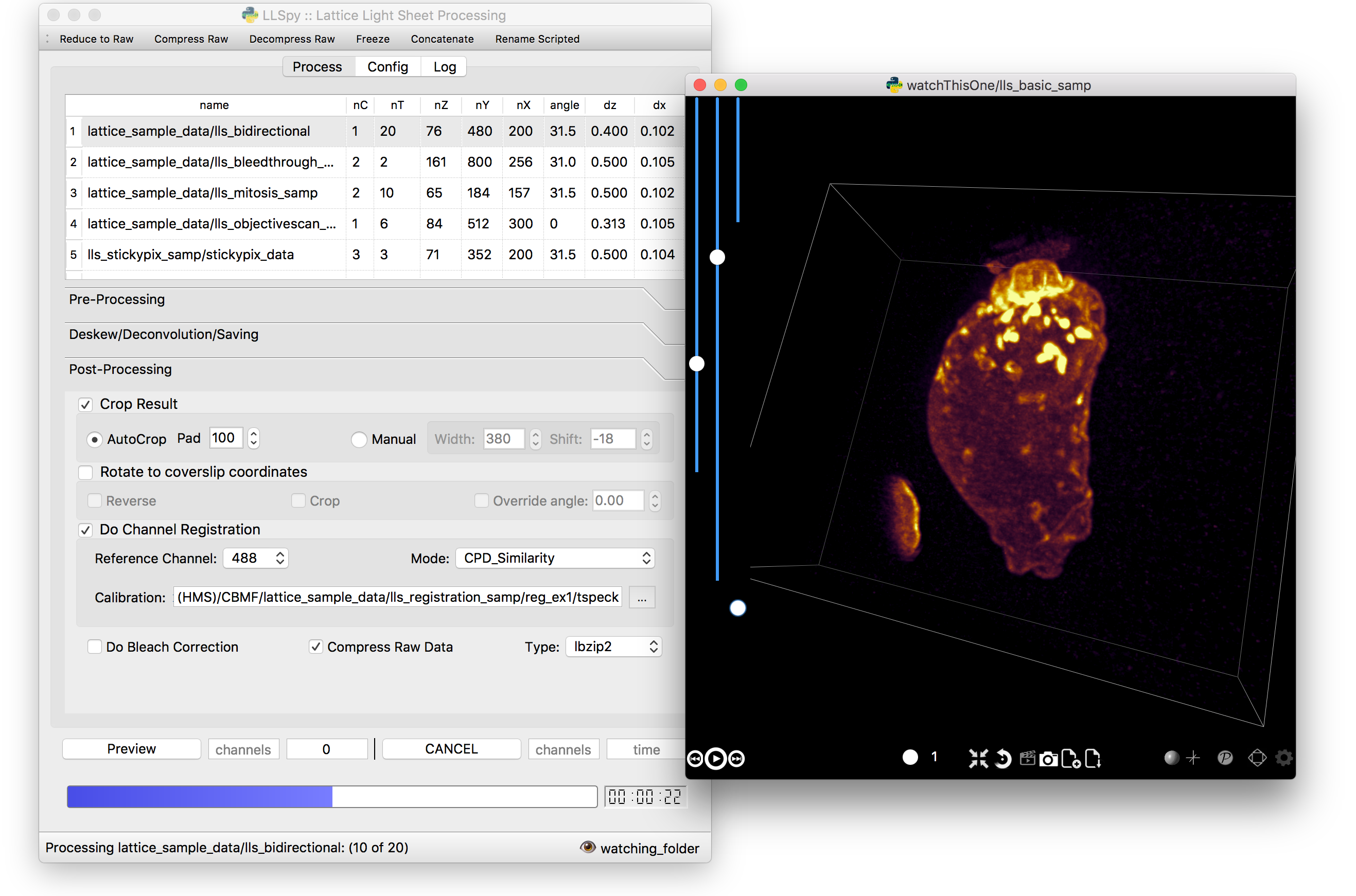
Process Tab

This tab has all of the settings for cudaDeconv and associated processing routines.

Folder Queue ListBox

Drag and drop LLS folders into the table (blank) area towards the top of the process tab to add them to the processing queue. Folders without a settings.txt file will be ignored. Basic experimental parameters are parsed from Settings.txt and folder structure and displayed. Future option may allow overwriting angle, dz, and dx in this list.

Pre-Processing

Most of these options pertain to image corrections or modifications prior to processing with cudaDeconv.

Camera Corrections

Checking the “Do Flash Correction” button to enable correction of the residual electron artifact seen in the Flash4.0 when using overlap/synchronous readout mode as is commonly done in the Lattice Scope software. In this readout mode, pixels in the chip are not reset between exposures causing “carryover” charge from the previous exposure in the next exposure. This can be seen as a noisy ghosting artifact in the second image in regions that were bright in the first image, which becomes particularly noticeable in deskewed and max projected images.

For correction, a calibration image must be specified in the “Camparam Tiff” field. This file is a tiff that holds parameters that describe the probability of carryover charge for each pixel (as a function of the intensity of that pixel in the previous image), along with the pixels specific offset (and optionally, noise). This can be used to subtract the predicted carryover charge, minimizing the artifact. Much more information availble here: LLSpy Camera Corrections

Camera correction can be done serially in a single thread on the CPU (CPU), with multithreading (parallel), or on the GPU (CUDA).

The “Do Median Filter” option will additionally replace particularly noisy pixels with the median value of its 8 neighboring pixels. For more information see the supplement in Amat et al. 2015.

Amat, F., Höckendorf, B., Wan, Y., Lemon, W. C., McDole, K., & Keller, P. J. (2015). Efficient processing and analysis of large-scale light-sheet microscopy data. Nature Protocols, 10(11), 1679–1696. http://doi.org/10.1038/nprot.2015.111 http://www.nature.com/nprot/journal/v10/n11/abs/nprot.2015.111.html

If “Save Corrected” is checked, the corrected pre-processed images will be saved. Otherwise, they are deleted after processing to save space.

Trim Edges

These settings allow you crop a number of pixels from each edge of the raw data volume prior to processing.

Sometimes when imaging a subregion of the chip on a CMOS camera, the last 1 or 2 rows on the edge will be particularly bright, especially if there is a bright object just outside of the ROI. After deskewing and max projection, those bright edges often corrupt the image. Use Trim X Left and Trim X Right to crop pixels on the sides of the images prior to processing.

Sometimes, when the camera has not taken an image in a while, dark current will accumulate in the photodiodes that causes the first image in a stack to appear noisier (this phenomenon again depends on using synchronous/overlap triggering mode). This noise will corrupt a max-intensity image. Setting “Trim Z first” to 1 or 2 is usually sufficient to remove the noise (though, obviously, will eliminate any data in those planes as well).

Trimming in the Y direction is mostly used to simply crop excess pixels from the image to save space.

Background Subtraction

In addition to a manually set “Fixed Value”, there is an option to “Autodetect” the background for each channel. In this case, the mode value of the second image in the z stack is used as the background value for that channel.

Deskew/Deconvolution/Saving

These options dictate what processing should be done, and what should be saved.

Deconvolution

If “Do Deconvolution” is checked and Iterations is greater than zero, deconvolution will be performed. nApodize and nZblend directly control the corresponding parameters in cudaDeconv.

“Save MIPs” check boxes determine which axes will have maximum-intensity-projections generated.

The 16-bit / 32-bit dropdown menu controls the bit-depth of the resulting deconvolved files.

Raw Deskewed

If “Save Deskewed” is checked, the raw (non-deconvolved) deskewed files will be saved. Note: for experiments acquired in galvo/piezo scanning mode (i.e. not in sample-scan), this section does nothing.

“Save MIPs” check boxes determine which axes will have maximum-intensity-projections generated.

The 16-bit / 32-bit dropdown menu controls the bit-depth of the resulting deconvolved files.

Join MIPS into single hyperstack

This option applies to both Deskewed and Deconvolved MIP folders, and combines all of the tiff files in each of those folders into a single multichannel/timelapse hyperstack that will be recognized by ImageJ/Fiji.

Post-Processing

While many of these options are technically performed during processing by the cudaDeconv binary, they all fall into the category of things done to the image after deconvolution/deskewing has already been performed.

Cropping

The “Crop Result” checkbox will crop the resulting deskewed/deconvolved image (in the X direction only). “AutoCrop” will automatically select a crop region based on image feature content. This is done by processing all channels from the first and last timepoints, and summing their max-intensity projections prior to heavy gaussian blurring. That summed & blurred image is segmented and a bounding box is calculated that contains the features in the image. The “Pad” setting adds additional pixels to both sides of the calculated bounding box.

Whether or not AutoCrop is chosen, the “Preview” button can be used to preview and evaluate the current settings in the processed image. If the Preview button is clicked when the AutoCrop option is selected, the autodetected “Width” and “Shift” values will be appear in the “Manual” cropping settings to the right where they can be further tuned and previewed prior to processing.

Rotate to coverslip

Rotate and interpolate data so that the Z axis of the image volume is orthogonal to the coverslip (does nothing beyond what cudaDeconv does).

Channel Registration (experimental)

When “Do Channel Registration” is checked, the deskewed/deconvolved data will be registered using the provided registration file or calibration folder, specified in the “Calibration” text field. If providing a calibration folder, it should contain at least one Z-stack, for each channel, of a fiducial marker that appears in all channels, such as tetraspeck beads. The folder must also contain a Settings.txt file (simply acquiring more than one timepoint is an easy way to generate an appropriate folder). A preferable method is to provide a pre-calculated registration file. Please read more in the Introduction to Channel Registration section.

Bleach Correction

Enables setting in cudaDeconv to normalize all timepoints to the intensity of the first timepoint, minimizing the appearance of photobleaching over the course of the timelapse, but altering the intensity values of the resulting deskewed/deconvolved images.

Compress Raw Data

After processing, compress the raw data using lbzip2 parallel compression.

Preview Button

Note: Documentation below currently only applies to the “matplotlib” viewer… not the spimagine viewer.

The Preview button (Ctrl-P) is used to process and show the first timepoint (by default) of the dataset selected in the processing queue, allowing evaluation of the current settings prior to processing of the entire folder. After clicking “Preview”, a multidimensional image window will appear after a moment of processing. This window has a number of features (some non-obvious):

• hovering over the image will show the coordinate and intensity value of the pixel under the mouse.
• use the Magnifying glass icon and up/down/left/right icon to zoom and pan, respectively.
• use the Z slider or the mouse wheel to select the Z plane to show
• use the C slider to change the currently displayed channel
• the min/max sliders adjust scaling of the image
• click on the colorbar to the right, or press the “C” key to cycle the colormap through some LUTs.
• Press the following keys for various projections. To return to standard Z-scrolling mode, press the same key again.
  • M - Max intensity projection
  • N - Min intensity projection
  • B - Mean intensity projection
  • V - Standard Deviation intensity projection
  • , - Median intensity projection
• To overlay multiple channels, click the “Overlay” button or press the “O” key on the keyboard. You may then select the color and contrast for each channel.

To preview multiple timepoints, or something other than the first timepoint, use the time subset field, which accepts a comma seperated string of (zero-indexed) timepoints, or ranges with start-stop[-step] syntax.

For instance:

• 0-2,9 - process the first three and 10th timepoints.
• 1-5-2 - start-stop-step syntax, processes the 2nd, 4th, and 6th timepoints
• 0,2-4,7-15-3 - combination of list, range, and range-with-step syntax

Process Button

The Process button (Ctrl-R) is used to process the entire dataset (by default) using cudaDeconv with the currently selected options.

To process a subset of timepoints or channels, use the time subset and channel subset fields, which accept a comma seperated string of (zero-indexed) timepoints, or ranges with start-stop[-step] syntax.

For instance:

• 0-2,9 - process the first three and 10th timepoints.
• 1-5-2 - start-stop-step syntax, processes the 2nd, 4th, and 6th timepoints
• 0,2-4,7-15-3 - combination of list, range, and range-with-step syntax

Config Tab

Use bundled cudaDeconv Binary

By default the program will use bundled cudaDeconv binaries, autoselecting based on the operating system. Tested on OS X, Linux, and Windows 7/10.

cudaDeconv binary

Unselect the “Use bundled cudaDeconv binary” option to enable this field which will allow you to specify the path to a specific cudaDeconv binary. Note: many of the features in LLSpy assume that the bundled binary is used. However, an attempt has been made to accomodate any binary by detecting the available options in the help menu, and disabling any non-matching features from LLSpy. However, this is still experimental, and may cause unexpected issues.

OTF directory and OTF auto-selection

Path to the folder that holds OTF and PSF files.

As a fallback, the program will look in this path for an otf file that is labeled [Wavelength]_otf.tif For example: 488_otf.tif

Before using the default otf, the program will attempt to find an appropriate PSF/OTF file to use based on the date of acquisition of the experiment, the mask used (provided the mask has been entered into SPIMProject.ini, see below), and the wavelength. Currently, files in the OTF directory must have the following format:

[date]_[wave]_[psf-type][outerNA]-[innerNA].tif

for example: 20170103_488_totPSFmb0p5-0p42.tif or 20170103_488_totPSFmb0p5-0p42_otf.tif

If a matching PSF file is found that does not have an OTF file already generated, it will generate an OTF file and save it with the _otf.tif suffix. This allows you to simply acquire a PSF file, and drop it in the PSF folder with the appropriate naming convention, and an OTF will automatically be generated when that PSF is used.

In order to select and OTF based on mask pattern, the mask must be in the Settings.txt file in the experiment. The easiest way to do this is to add an “Annular Mask” section to the SPIMProject.ini file in the Lattice Scope software, and update the values each time you change the mask. For instance:

[Annular Mask]
outerNA = 0.5
innerNA = 0.42

Generating Camera Calibration File

The calibration algorithm assumes that you have aquired a series of 2-channel Zstacks (not actually a 3D stack: set Z galvo range and Z and Sample Piezo range to zero). The first channel should be “bright” (many photons hitting the chip) and even like a flatfield image (such as 488 laser sheet exciting FITC) and the second channel is a “dark” image (I use another wavelength channel with the laser off. Collect two ~100-plane Z stacks for many different intensities (laser power) in the “bright channel”: start at very low power (0.1% laser) and gradually acquire stacks at higher power. Due to the exponential relationship of the residual electron effect, it’s particularly important to get a lot of low-powered stacks: 1%, 2%, 3% etc… then after 10% you can begin to take bigger steps. (Of course, the exact laser powers will depend on the power and efficiency of your system.

Upon clicking the “Generate Camera Calibration File” button, select the path to the folder that contains all of the bright/dark images acquired above. By default, the program will look for an image called Dark_AVG.tif in the selected Image Folder, but the average projection image can also be manually selected. Optionally, a standard deviation projection of the dark image stack (i.e. noise map) can be also provided in the same folder, named Dark_STD.tif, and it will be included in the calibration file.

Even with parallel processing, this process takes a while: about ~30 minutes for a 1024x512 ROI on a computer with a 4 core, 4 GHz processer (i7-6700K). However, it should only need to be calculated once. I have been using the same correction file for about a year, and it continues to be appropriate for my camera.

The output file will appear in the Image Folder. Put it somewhere you will remember and enter the path on the Config Tab in the LLSpy GUI.

Reprocess folders that have already been processed

If left unchecked, LLSpy will skip over any folders that have already been processed (i.e. folders that already contain a ProcessingLog.txt file)

Save MIP Folder during “Reduce to Raw”

The “Reduce to Raw” shortcut in the toolbar deletes any GPUdecon, Deskwed, Corrected, and MIP folders, restoring folder to state immediately after aquisition. This option in the config tab alters the behavior of the “reduce” function to leave any MIP folders for easy preview in the future.

Warn when quitting with unprocessed items

By default, LLSpy will warn you if you have unprocessed items remaining in the queue. Turn this option off here.

Preview Type

Choose between a standard single-plane viewer (with various projection modes), and the Spimagine 4D viewer.

Watch Directory (experimental)

These options designate a folder to watch and auto-process when a new LLS folder appears.

Watch Modes

• Server mode: designate a folder to watch for incoming finished LLS folders (with Settings.txt) file. When new folders are detected, they are added to the processing queue and the queue is started if not already in progress.
• Aquisition mode: designed to be used on the aquisition computer. Designate folder to watch for new LLS folders, and process new files as they arrive. Similar to built in GPU processing tab in Lattice Scope software, but with the addition of all the corrections and parameter selection in the GUI.

Error reporting Opt Out

In order to improve the stability of LLSpy, crashes and uncaught exceptions/errors are collected and sent to sentry.io. These bug reports are extremely helpful for improving the program. No personal information is collected, and the full error-reporting logic may be inspected in llspy.gui.exceptions. However, you may opt out of automatic error reporting with this checkbox.

Log Tab

Any output from cudaDeconv or LLSpy will appear in this tab. Note: a program log is also written to disk, the location of this file varies with OS. On mac it is in the Application Support folder. On windows, it is in the %APPDATA% folder.

Progress and Status Bar

During cudaDeconv processing, the current file number will appear in the status bar at the bottom of the window, and the percent progress is represented by the progress bar. The timer countdown on the right provides an estimate of the time remaining for the current LLS directory (not for the entire queue). If a folder is being monitored for new data, it will show up at the bottom right corner of the status bar.

Command Line Interface

In addition to the QT-based graphical user interface, LLSpy includes a command line interface (CLI).

If the program has been installed using conda install -c talley -c conda-forge llspy, or by using setuptools (i.e. running pip install . in the top level llspy directory, where setup.py resides) then an executable will be created that can be triggered by typing lls at the command prompt. Alternatively, the CLI can be directly executed by running python llspy/bin/llspy_cli.py at the command prompt. (For this documentation, it is assumed that the program was installed using conda install and run with lls).

$ lls --help
Usage: lls [OPTIONS] COMMAND [ARGS]...

  LLSpy

  This is the command line interface for the LLSpy library, to facilitate
  processing of lattice light sheet data using cudaDeconv and other tools.

Options:
  --version          Show the version and exit.
  -c, --config PATH  Config file to use instead of the system config.
  -h, --help         Show this message and exit.

Commands:
  camera    Camera correction calibration
  compress  Compression & decompression of LLSdir
  config    Manipulate the system configuration for LLSpy
  decon     Deskew and deconvolve data in LLSDIR.
  deskew    Deskewing only (no decon) of LLS data
  gui       Launch the Graphical User Interface.
  info      Get info on LLSDIR.
  reg       Channel registration

You can configure the program either by providing a configuration .ini in the command using the --config flag, or by setting the system configuration using the llspy config command. Minimally, you will want to establish the OTF directory by typing:

$ lls config --set otfDir /path/to/OTFs/

To get a full list of keys available for configuration, type:

$ lls config --info

To print the current system configuration, type:

$ lls config --print

Note: System configuration values will be superceeded by key-value pairs included in config.ini files provided at the command prompt with --config, and all configuration values will be superceeded by those privided directly using option flags in the decon command.

You can use --help to get more information on any specific subcommand. Many are still under development. The bulk of the program functionality resides in the decon subcommand.

$ lls decon --help
Usage: lls decon [OPTIONS] LLSDIR

  Deskew and deconvolve data in LLSDIR.

Options:
  -c, --config PATH              Overwrite defaults with values in specified
                                 file.
  --otfDir DIRECTORY             Directory with otfs. OTFs should be named
                                 (e.g.): 488_otf.tif
  -b, --background INT           Background to subtract. -1 = autodetect.
                                 [default: -1]
  -i, --iters [INT: 0-30]        Number of RL-deconvolution iterations
                                 [default: 10]
  -R, --rotate                   rotate image to coverslip coordinates after
                                 deconvolution  [default: False]
  -S, --saveDeskewed             Save raw deskwed files, in addition to
                                 deconvolved.  [default: False]
  --cropPad INT                  additional edge pixels to keep when
                                 autocropping  [default: 50]
  -w, --width [INT: 0-3000]      Width of image after deskewing. 0 = full
                                 frame.[default: autocrop based on image
                                 content]
  -s, --shift [INT: -1500-1500]  Shift center when cropping  [default: 0]
  -m, --rMIP <BOOL BOOL BOOL>    Save max-intensity projection after
                                 deskewing along x, y, or z axis.  Takes 3
                                 binary numbers separated by spaces.
                                 [default: False, False, False]
  -M, --MIP <BOOL BOOL BOOL>     Save max-intensity projection after
                                 deconvolution along x, y, or z axis. Takes 3
                                 binary numbers separated by spaces  [default:
                                 False, False, True]
  --mergemips / --sepmips        Combine MIP files into single hyperstack (or
                                 not).  [default: True]
  --uint16 / --uint32            Save results as 16 (default) or 32- bit
  -p, --bleachCorrect            Perform bleach correction on timelapse data
                                 [default: False]
  --trimX <LEFT RIGHT>           Number of X pixels to trim off raw data
                                 before processing  [default: 0, 0]
  --trimY <TOP BOT>              Number of Y pixels to trim off raw data
                                 before processing  [default: 0, 0]
  --trimZ <FIRST LAST>           Number of Z pixels to trim off raw data
                                 before processing  [default: 0, 0]
  -f, --correctFlash             Correct Flash pixels before processing.
                                 [default: False]
  -F, --medianFilter             Correct raw data with selective median
                                 filter. Note: this occurs after flash
                                 correction (if requested).  [default: False]
  --keepCorrected                Process even if the folder already has a
                                 processingLog JSON file, (otherwise skip)
  -z, --compress                 Compress raw files after processing
                                 [default: False]
  -r, --reprocess                Process even if the folder already has a
                                 processingLog JSON file, (otherwise skip)
  --batch                        batch process folder: Recurse through all
                                 subfolders with a Settings.txt file
  --yes / --no                   autorespond to prompts
  -h, --help                     Show this message and exit.

Developer Interface

This part of the documentation covers the interfaces of LLSpy that one might use in development or interactive sessions. This page is a work in progress: there is much more undocumented functionality in the source code.

Main Functions

Processing routines can be called directly with a path to the LLS experiment directory.

Main Classes

Most routines in LLSpy begin with the instantiation of an LLSdir object. This class is also instantiated by the preview and process functions

LLS directory

cudaDeconv wrapper

*Settings.txt parser

Wrapped CUDA functions

Exceptions

Schema

Many functions such as the preview and process functions accept keyword arguments that determine processing options. These are all validated using the schema in llspy.schema. Options include:

Key	Default	Description
correctFlash	False	do Flash residual correction
moveCorrected	True	move processed corrected files to original LLSdir
flashCorrectTarget	cpu	{“cpu”, “cuda”, “parallel”} for FlashCor
medianFilter	False	do Keller median filter
keepCorrected	False	save corrected images after processing
trimZ	(0, 0)	num Z pix to trim off raw data before processing
trimY	(0, 0)	num Y pix to trim off raw data before processing
trimX	(0, 0)	num X pix to trim off raw data before processing
nIters	10	deconvolution iters
nApodize	15	num pixels to soften edge with for decon
nZblend	0	num top/bot Z sections to blend to reduce axial ringing
bRotate	False	do Rotation to coverslip coordinates
rotate	None	angle to use for rotation
saveDeskewedRaw	False	whether to save raw deskewed
saveDecon	True	whether to save decon stacks
MIP	(0, 0, 1)	whether to save XYZ decon MIPs
rMIP	(0, 0, 0)	whether to save XYZ raw MIPs
mergeMIPs	True	do MIP merge into single file (decon)
mergeMIPsraw	True	do MIP merge into single file (deskewed)
uint16	True	save decon as unsigned int16
uint16raw	True	save deskewed raw as unsigned int16
bleachCorrection	False	do photobleach correction
doReg	False	do channel registration
regRefWave	488	reference wavelength when registering
regMode	2step	transformation mode when registering
regCalibPath	None	directory with registration calibration data
mincount	10	minimum number of beads expected in regCal data
reprocess	False	reprocess already-done data when processing
tRange	None	time range to process (None means all)
cRange	None	channel range to process (None means all)
otfDir	None	directory to look in for PSFs/OTFs
camparamsPath	None	file path to camera Parameters .tif
verbose	0	verbosity level when processing {0,1,2}
cropMode	none	{manual, auto, none} - auto-cropping based on image content
autoCropSigma	2	gaussian blur sigma when autocropping
width	0	final width when not autocropping (0 = full)
shift	0	crop shift when not autocropping
cropPad	50	additional pixels to keep when autocropping
background	-1	background to subtract. -1 = autodetect
compressRaw	False	do compression of raw data after processing
compressionType	lbzip2	compression binary {lbzip2, bzip2, pbzip2, pigz, gzip}
writeLog	True	write settings to processinglog.txt

LLSpy Camera Corrections

All sCMOS cameras demonstrate pixel-specific noise, gain, and offset characteristics. For a basic understanding of camera parameters, see my chapter on assessing camera performance. For an updated look at sCMOS-specific issues, I recommend looking through the supplementary methods of Fang Huang’s two papers on sCMOS corrections. The Flash4.0 used on many lattice scopes is further prone to a specific artifact that becomes very apparent when combined with stage-scanning acquisition and deskewing (the smeared, horizontal, repeating patterns in the image shown below). This page describes the artifact and outlines a method for camera-specific calibration and correction of the problem.

Fig 1. Maximum intensity projection of a deskewed 3D volume. The faint, repeating horizontal “noisy” pattern is a result of a camera artifact seen on the Flash4.0 when used in synchronous readout triggering mode.

Synchronous readout mode

The Flash4.0 offers a fast readout mode called synchronous readout external trigger mode, in which the camera exposure is ended, readout is started and the next eposure is simultaneously started by the edge of an external (TTL) trigger signal input to the camera. This technical note released for the Flash4.0 V2 describes the various triggering modes on pages 16-17 (it also applies to Flash4.0 V3), with synchronous readout shown in Fig 32. The Janelia acquisition software uses synchronous readout mode to trigger camera readout during SLM pattern reloading to optimize acquisition speed. Unlike the other external trigger modes, synchronous readout does not include a “reset”, where the charge is reset in each pixel after readout (see Fig 12 in the technical note). As a result, there is a possibility that “residual” charge will carry over in a given pixel from one exposure to the next. This carryover charge is particularly noticeable when there is a bright object in one channel but not in the second channel, as shown in the image below. The magnitude and probability of charge carryover is pixel-specific: some pixels are more prone to charge carryover than others.

Fig 2. Raw data acquired in stage scanning mode on the lattice. Residual charge from the bright object in channel 2 can be seen as noisy/brighter pixels in channel 1. Images are scaled identically.

After Deskewing…

In a conventional acquisition scheme, where the image plane is orthogonal to the axis of Z-motion, this artifact would perhaps be a bit less noticeable. However, when a dataset acquired in stage-scanning mode is deskewed and max-projected, the carryover charge in the problematic pixels gets “smeared” across the X dimension in the resulting volume, and becomes very apparent in a maximum-intensity projection.

Fig 3. Carryover charge in a given pixel on the camera becomes smeared across the X dimension after deskewing, and is partiucularly apparent in a maximum-intensity projection.

(If it’s unclear why data acquired in stage-scanning mode needs to be deskewed, see this video)

Camera Characterization and Correction

Fortunately, the probability of charge carryover in a given pixel is constant over time, and can be relatively well modeled. To characterize your particular camera, you need to create a dataset that allows you to measure the magnitude of charge carryover in every pixel. One way to do this is to collect a series of alternating “bright” and “dark” exposures, where the bright image has even illumination across the chip and the dark image receives zero photons. By collecting thousands of these image-pairs while gradually increasing the intensity of the bright image that precedes the dark image, you can map the relationship between intensity of any given pixel in one exposure and the carryover intensity in the following exposure. An example of such a calibration dataset collected on the lattice is shown in the top row of figure 4 below: where the “bright image” on the left is a flat-field image acquired by illuminating a fluorescein solution with a dithered sheet, and the image on the right is a “dark image” that was aquired using zero illumination light (and confirming that no background room-light contamination can reach the chip).

Fig 4. Carryover charge characterization data. The top shows raw data collected on the lattice: the “bright image” (ch0) on the left is acquired by illuminating a fluorescein solution with a dithered sheet, and the image on the right is a “dark image” (ch1) that was aquired in a second channel using zero illumination light. The top row shows the same dataset after the carryover correction has been applied. Intensity values in each are indicated in the lookup table plots.

By plotting the intensity in exposure 2 as a function of exposure 1 for many thousands of images at varying levels of brightness in exposure 1, the relationship between intensity in exposure 1 and carryover in exposure 2 becomes clear. Example data from a single pixel is shown below in figure 5 (note: pixel-specific camera offset has been subtracted from both images.)

Fig 5. Calibration data from a single pixel showing the relationship betwen the intensity of an image and carryover charge in the immediately following image

The parameters describing the probability of charge carryover for a given pixel can be extracted by fitting these data to an exponential association curve. This is repeated for every pixel on the chip. The resulting parameters can be used to correct an experimental dataset by subtracting the predicted carryover charge in any given image as a function of the intensity of the previous image. The reduction of carryover charge after this correction can be seen in “dark image” in the bottom row of figure 4, where the correction has been applied to the calibration dataset itself, leaving mostly just read noise.

An example with experimental data is shown below, where the correction has been applied to the data from Figure 2.

Fig 6. Deskewed maximum intensity projection of data shown in Figure 2, before and after carryover charge correction. (bright second-channel image not shown).

Note

When running the Lattice Scope software in twin-cam mode, it is usually not necessary to perform charge carryover correction. In twin-cam mode, both cameras are triggered during every camera-fire trigger (for example: the camera collecting green emission photons takes an image during both the 488nm laser pulse as well as the 560nm pulse). This “non-matching” image (i.e. the green-camera image taken during the 560nm laser pulse) is not usually saved by the software, but it does “clear” the residual charge carryover from the previous image, effectively resetting the pixel charge before the next exposure.

LLSpy Carrover Correction

LLSpy provides two convenience features:

1. An interface to generate your own camera correction file from a folder of bright/dark images you have collected.
2. A function to apply the correction to your experimental data, extracting ROI information from the settings.txt file to match pixels in the raw data to corresponding pixels in the correction file.

Camera Calibration in LLSpy

To correct carryover charge in your images, you must first collect a dataset of alternating bright/dark images as described above in Camera characterization and correction. Fluorescein in solution is useful to create a relatively even “bright” image, but any even-illumination scheme where you can alter the intensity of the illumination will work. Set up a two-channel acquisition, where the first channel is “bright” (e.g. a dithered square lattice and 488nm laser exciting fluorescein solution) and the second channel is “dark” (e.g. no laser illumination at all, room lights blocked from camera chip). Use a camera ROI that is at least as large as the largest dataset that you would like to correct. I use an ROI of 1024 x 512, which is larger than pretty much all of image sizes I tend to collect. Gradually increase the intensity of the bright-channel laser intensity, and collect about 200 of these two-channel images at each intensity. Ideally, you want to have image-pairs with bright-channel intensities ranging from nothing (just camera offset) to ~5000 intensitiy values (see figure 5, where each point in the graph represents a single image-pair). Start at very low power (0.1% laser) and gradually acquire stacks at higher power. Due to the exponential relationship of the residual electron effect, it’s particularly important to get a lot of low-powered stacks: 1%, 2%, 3% etc… then after 10% you can begin to take bigger steps. The exact laser power and exposure times will obvious depend on the power of your laser and the concentration of fluorescein used, so you will need to determine them empirically. I use the Script Editor feature in the Lattice Scope software to iteratively collect ~200 images, then raise the 488 laser power and repeat, etc…

In addition to the bright-dark image-pairs, you will need to collect >20,000 dark-only images that will be used to estimate the per-pixel camera noise and offset (only offset is used for the carryover charge correction, but having the noise map as well is useful and may be used by LLSpy in the future). The ROI used when collecting these images must be the same as when collecting the bright-dark image-pairs.

It is also important that there be at least one Settings.txt file in the directory that will be used to detect and store the camera serial number and the ROI used for calibration (which is critical for later alignment with experimental data). An example of a typical calibration folder structure is shown below.

/calibration_folder/
├── bright00p1_Iter_CamA_ch0_stack0000_488nm.tif
├── bright00p1_Iter_CamA_ch1_stack0000_642nm.tif
├── bright00p1_Iter_Settings.txt
├── bright00p2_Iter_CamA_ch0_stack0000_488nm.tif
├── bright00p2_Iter_CamA_ch1_stack0000_642nm.tif
├── bright00p2_Iter_Settings.txt
├── bright00p4_Iter_CamA_ch0_stack0000_488nm.tif
├── bright00p4_Iter_CamA_ch1_stack0000_642nm.tif
├── bright00p4_Iter_Settings.txt
.
.
.
├── bright80p0_Iter_CamA_ch0_stack0000_488nm.tif
├── bright80p0_Iter_CamA_ch1_stack0000_642nm.tif
├── bright80p0_Iter_Settings.txt
├── bright90p0_Iter_CamA_ch0_stack0000_488nm.tif
├── bright90p0_Iter_CamA_ch1_stack0000_642nm.tif
├── bright90p0_Iter_Settings.txt
.
.
.
├── dark_Iter_CamA_ch0_stack0000_488nm.tif
├── dark_Iter_CamA_ch0_stack0001_488nm.tif
├── dark_Iter_CamA_ch0_stack0002_488nm.tif
.
.
.

Note

Don’t confuse the ~20,000 “dark images” used for estimating camera offset with the “dark images” (ch1) that immediately follow the “bright images” (ch0) in each image-pair with gradually increasing laser intensity. In the example below, everything that has ch1_stack0000_642nm.tif in the name is a dark image used for estimating carryover charge (the 642nm laser wasn’t on), whereas everything that has the word dark in the filename will be averaged together to measure camera offset. The only thing LLSpy cares about is the word “dark” in the filename. It will use those for offset measurement, and everything else is assumed to be a bright/dark (ch0/ch1) matched image-pair.

Note

A small example dataset for calibration can be downloaded here. For actual characterization, you should use more images than the number provided in the sample data.

Once you have gathered the data, you can generate the camera correction file using either the command line tool:

$ lls camera -c /path/to/calibration_folder/

or the “Camera Calibration” window in the LLSpy GUI, which can be found in the Tools menu.

In the GUI window, click the Select Folder button next to the Image Folder field and navigate to the folder containing your calibration data. Note, you may optionally provide pre-calculated dark average (AVG) and standard deviation (STD) projection images. But if you simply include the raw dark images in the calibration folder and put the word “dark” in their filenames (as shown above in the example folder structure), those files will be used to calculated the AVG and STD projection images for you. This is recommended (and it is required when using the command line interface, where you cannot provide the AVG and STD projections seperately). Click the Run button and the program will calculate correction file. This may take quite a while (many hours even) depending on your system, but the progress bar will provide a time estimate after a short delay. Currently, the only way to stop the process is just to quit LLSpy (simply closing the window will not stop the process). Once done, the program will output the correction file into the same folder used for calibartion. Find this file (it will be labeled something like FlashParam_sn{}_roi{}_date{}.tif) and store it somewhere you will remember.

Applying the Correction in LLSpy

Once you have generated the camera correction file, you can use it to correct your experimental data. In the LLSpy GUI, on the Process tab, in the “Pre-Processing” section, click the ... button next to the “CameraParam Tiff” field and select your camera correction tiff that you previously generated. To apply the correction check the “Do Flash Correction” checkbox. You may then select whether the correction is calculated single-threaded on the CPU, multithreaded in parallel on the CPU, or on the GPU using CUDA. For most purposes, parallel correction is the fastest (but CUDA is similarly fast).

If using the command line interface for LLSpy, you need to set your configuration to use the newly generated file as follows:

$ lls config --set camparamsPath /path/to/FlashParam.tif

and (optionally) set the hardware target for performing the correction, for example:

$ lls config --set flashCorrectTarget parallel

Selective Median Filter

The “Do Median Filter” option will replace particularly noisy pixels with the median value of its 8 neighboring pixels. The method can be briefly summarized as follows:

1. Calculate standard deviation projection of the raw Z stack (devProj)
2. Median filter the deviation projection (devProjMedFilt)
3. Take the difference between devProj and devProjMedFilt (deviationDistance)
4. Find pixels whose deviationDistance is greater than some automatically determined threshold
5. Optionally repeat with Mean Projection… (which will detect pixels with aberrant gain)
6. In the original image, apply 3x3 median filter to all “bad” pixels above threshold

For more information see the supplement in Amat et al. 2015.

Amat, F., Höckendorf, B., Wan, Y., Lemon, W. C., McDole, K., & Keller, P. J. (2015). Efficient processing and analysis of large-scale light-sheet microscopy data. Nature Protocols, 10(11), 1679–1696. http://doi.org/10.1038/nprot.2015.111 http://www.nature.com/nprot/journal/v10/n11/abs/nprot.2015.111.html

This option can be used with or without the Flash Correction, and it does not require any pre-calibration of your camera. But as with all filters, it has the possibility to decrease the resolution of the image slightly (though it is a much less detrimental algorithm than simply applying a non-selective 3x3 median filter to the raw data). The method works particularly well when also applying the Flash correction first, as the number pixels that will be replaced by the selective median filter decreases dramatically.

Save Corrected

If “Save Corrected” is checked, the corrected pre-processed images will be saved. Otherwise, they are deleted after processing to save space.

Introduction to Channel Registration

Because almost all multi-channel images have some degree of channel misregistration (particularly on multi-camera setups), LLSpy includes a standard fiducial-based channel registration procedure. A calibration dataset is acquired with a sample of broad-spectrum diffraction limited objects (such as TetraSpeck beads). The objects are then detected and localized by fitting to a 3D gaussian model, yielding a set of 3D coordinates (X, Y, Z) for each object, for each channel. (In LLSpy, a single wavelength set of coordinates is instantiated by the fiducialreg.FiducialCloud class and a set of FiducialClouds is instantiated by the fiducialreg.CloudSet class). A transformation can then be calculated that maps (or ‘registers’) a set of coordinates for one channel (the “moving” set) onto a set of coordinates for another channel (the ‘reference’ set). Once calculated, that transformation matrix can then be used to register other data acquired in those two channels. (This of course assumes that nothing has changed in the microscope that would alter the spatial relationship between the images in those two channels… which is not always a safe assumption).

Transformation Modes

Contraints can be enforced when calculating transformation matrices, allowing varying degreese of freedom or “flexibility” when mapping one coordinate set onto another.

• Translation: simply corrects for translational shifts between channels
• Rigid: correct for translation and rotation differences
• Similarity: correct for translation, rotation, and scaling (magnification) differences.
• Affine: corrects translation, rotation, scaling, and shearing
• 2-step: performs affine registration in XY and rigid registraion in Z

When performing channel registraion, it is often beneficial to chose the “least flexible” transformation that “gets the job done”, as increasing degrees of freedom can sometimes lead dramatically bad registrations.

CPD Registration

The standard registration modes mentioned above require a one-to-one relationship between fidicual markers in each channel. LLSpy will therefore attempt to discard any coordinate points that do not have a corresponding point in both datasets being registered. Sometimes, that automated filtering fails, in which case the calculated registration will usually be nonsense. LLSpy also includes (experimental) support for Coherent Point Drift-based transformation estimation, using a slightly modified version of the pycpd library. For registration modes with ‘CPD’ prepended to the name, a one-to-one relationship between fiducial markers across channels will not be enforced. Please verify that your chosen registration mode correctly registers the fiducial dataset before applying it to experimental data, as described below in A Typical Workflow.

LLSpy Registration File

In LLSpy, you first create a Registration File (LLSpy.reg file) from a fiducial dataset, choosing the channels you may later want to use as the reference channel. Multiple transformations (e.g. translation, rigid, similarity, affine…) will be calculated that map all of the wavelengths in represented in the calibration data, to each of the reference wavelengths selected. The output file is in JSON format, an example is shown below:

{
  "tforms": [
    {
      "mode": "translation",
      "reference": 488,
      "moving": 560,
      "inworld": true,
      "tform": [
         [  1.0000000000,  0.0000000000,  0.0000000000,  0.0771111160],
         [  0.0000000000,  1.0000000000,  0.0000000000,  0.0138356744],
         [  0.0000000000,  0.0000000000,  1.0000000000,  0.5431871957],
         [  0.0000000000,  0.0000000000,  0.0000000000,  1.0000000000]
      ]
    },
    {
      "mode": "rigid",
      "reference": 488,
      "moving": 560,
      "inworld": true,
      "tform": [
         [  0.9999998846, -0.0004796165, -0.0000280755,  0.0771111160],
         [  0.0004796557,  0.9999988858,  0.0014136213,  0.0138356744],
         [  0.0000273975, -0.0014136346,  0.9999990004,  0.5431871957],
         [  0.0000000000,  0.0000000000,  0.0000000000,  1.0000000000]
      ]
    },
  ]
}

Using this template, you may also generate your own registration transformations using other software, and use them within LLSPy. Minimally, the registration file must have a top level dict ({ }) with a key tforms. The value of tforms must be a list of dict, where each dict in the list represents one transformation matrix. Each tform dict in the list must minimally have the following keys:

• mode: the type of registration performed. currently, must be one of the following:

  translation, translate, affine, rigid, similarity, 2step, cpd_affine, cpd_rigid, cpd_similarity, cpd_2step

• reference: the reference wavelength
• moving: the wavelength to be registered
• tform: the (forward) transformation matrix that maps the moving dataset onto the reference dataset. Must be a 4x4 matrix where the last row is [0,0,0,1].

The inworld key in the example JSON file above indicates that the pixel coordinates have been converted into real-world (i.e. microns X/Y instead of pixels) coordinates prior to calculation of the transformation. This is currently the default method in LLSpy, which should allow registration files to be used to register datasets whose voxel size differs from the fiducial calibration dataset used to generate the registration file.

A Typical Workflow

To perform registration in LLSpy, one will typically generate a registration file from a fiducial dataset, then apply the transformations in that file to experimental data. That file can be used until it is determined that the transformations no longer represent the channel-relationship in the data (the frequency with which the calibration must be performed will vary dramatically across systems and must be determined for your system.) To generate a registration file in the LLSpy gui, use the Registration tab, click the load button next to the Fidicual Data field, and select a folder containing multi-channel fiducial markers, such as tetraspeck beads. (Note: this folder must also include a settings.txt file. On the Lattice Scope software, the easiest way to generate a settings.txt file is simply to acquire more than one “timepoint”). Then select the Ref Channels to which you want to register, and click the Generate Registration File button. You will be prompted to select a destination for the file (a file will also be saved in your OS-specific application directory, such as %APPDATA%\LLSpy\regfiles on windows). The registration file will be automatically loaded into the Registration File field below, where you can then “test” out a given transformation mode and Ref Channel by registering the fiducal dataset itself, using the Register Fiducial Data button. Depending on the degree of channel misalignment, is very likely that some of the transformation modes will not work, so you should confirm which mode(s) worked in this window, before applying to experimental data. Finally, the registration file can be loaded in the main Process tab under the Post-Processing - Channel Registration section, by clicking the Use RegFile button, and selecting the desired Ref Wave and transformation Mode. If the Do Channel Registration checkbox is selected, that registration will then be applied to your deconvolved/deskewed data. Registered tiffs will have _REG appeneded to their filenames.

Indices and tables

• Index
• Module Index
• Search Page